
手撕自动驾驶算法——传感器融合算法:卡尔曼滤波器和扩展卡尔曼滤波器
·
传感器融合步骤
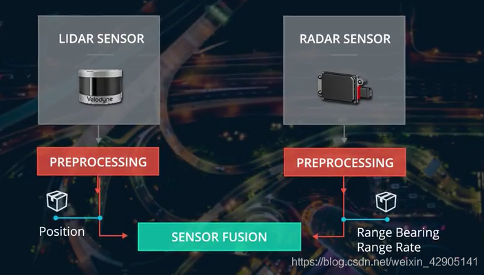
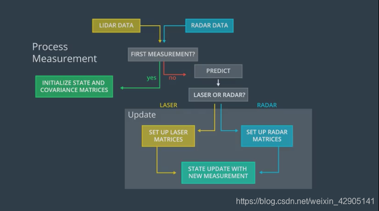
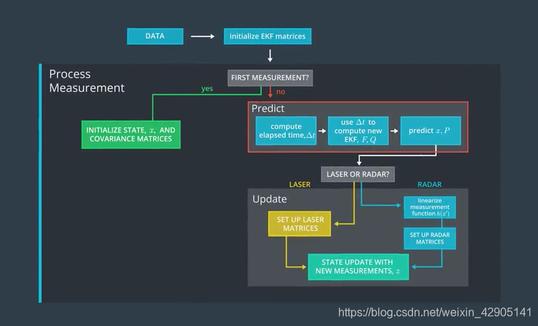 卡尔曼滤波器算法将执行以下步骤:
- 第一次测量 - 过滤器将接收自行车相对于汽车位置的初始测量值。这些测量将来自雷达或激光雷达传感器。
- 初始化状态和协方差矩阵 - 过滤器将根据第一次测量初始化自行车的位置。
- 然后汽车将在一段时间后接收另一个传感器测量值Δt\Delta{t}Δt。
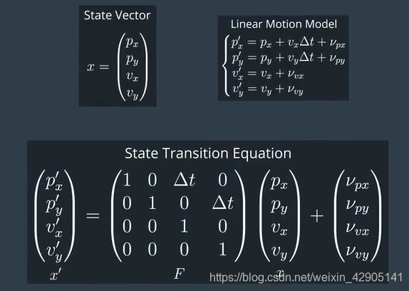
- 预测 - 算法将预测自行车在一段时间后的位置Δt\Delta{t}Δt。预测自行车位置的一种基本方法Δt\Delta{t}Δt是假设自行车的速度是恒定的; 因此自行车将移动速度Δt\Delta{t}Δt。在扩展卡尔曼滤波器课程中,我们假设速度是恒定的; 在无损的卡尔曼滤波器课程中,我们将介绍一个更复杂的运动模型。
- 更新 - 过滤器将“预测”位置与传感器测量值进行比较。将预测的位置和测量的位置组合以给出更新的位置。卡尔曼滤波器将根据每个值的不确定性对预测位置或测量位置施加更多权重。
- 然后汽车将在一段时间后接收另一个传感器测量值 Δt\Delta{t}Δt。然后该算法执行另一个预测和更新步骤。
1.使用激光雷达数据的基础卡尔曼滤波器
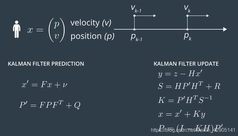
激光测量允许我们获取物体的当前位置而不是其速度。另一方面,激光测量具有更高的分辨率。
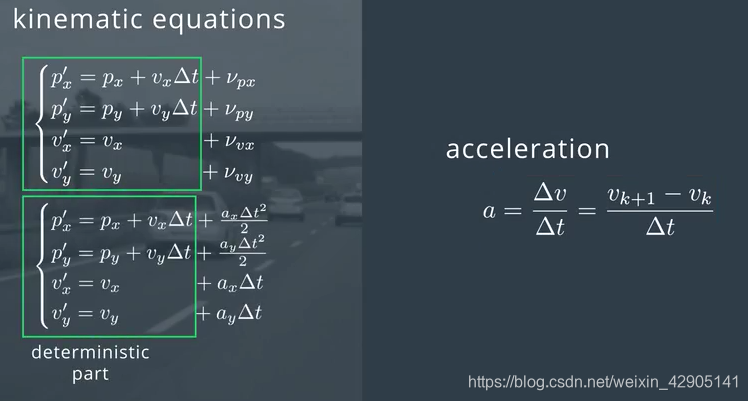
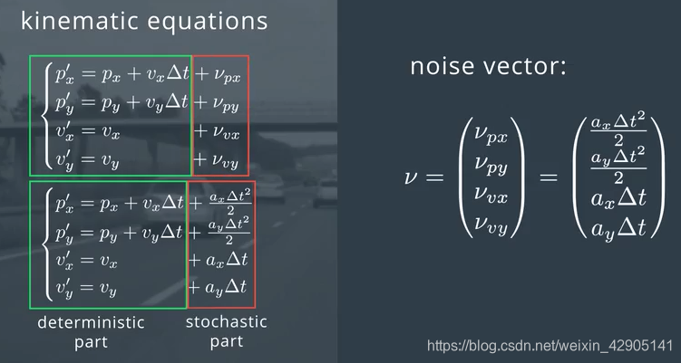
状态预测
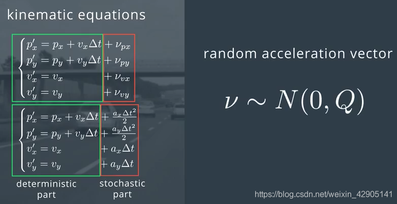
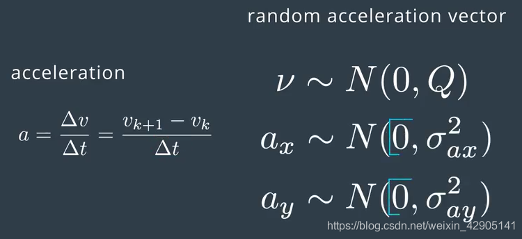
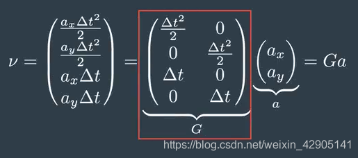
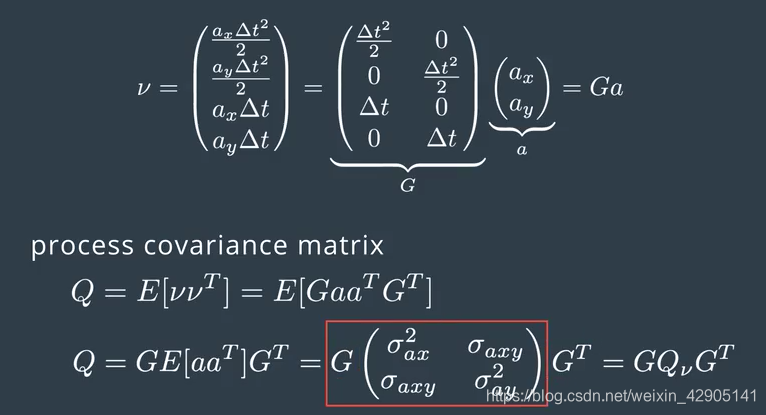
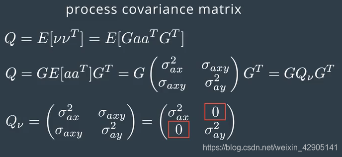
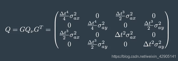
协方差矩阵Q
2.扩展卡尔曼滤波器——使用雷达数据
雷达数据带来了一些更困难的挑战。雷达返回数据值的是基于极坐标系,其由三个部分构成:
- ρ /Range(从原点到此的距离)
- ϕ / bearing ( ρ 和 x的夹角),
- ρ˙:接近率/距离变化率
由于没有H矩阵将状态向量映射到雷达的测量空间,我们需要一个函数h(x)来将状态空间银蛇到测量空间以测量更新步骤。这个方法是映射极坐标到笛卡尔坐标的方法的衍生方法,定义如下: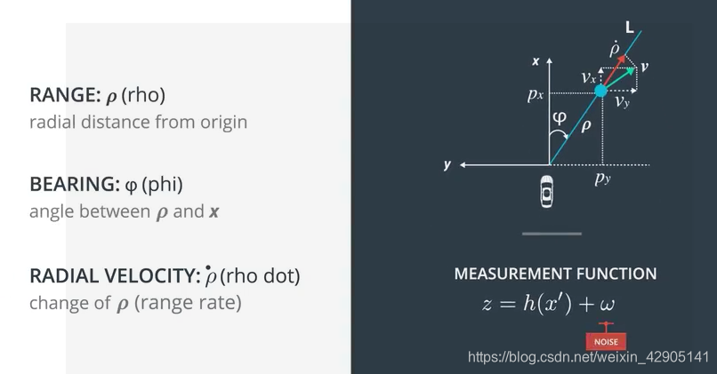
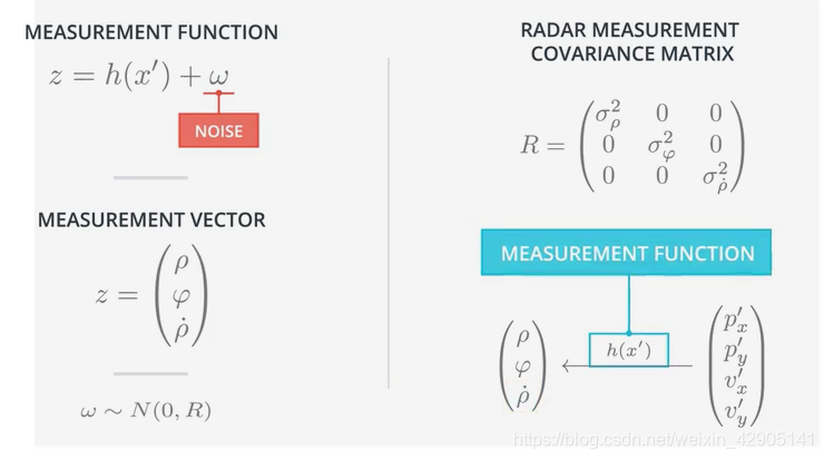
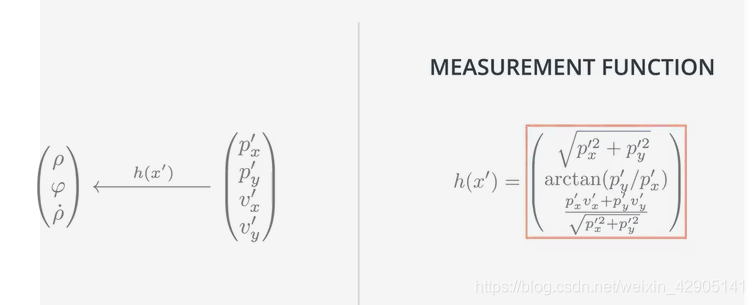
这个映射阐述了一个非线性函数,它将使得卡尔曼滤波器的过程和测量符合高斯分布的假设无效。扩展卡尔曼滤波器使用局部线性模型来逼近非线性模型,然后使用卡尔曼滤波应用到逼近值上。局部线性逼近是通过计算当前状态估计的一阶泰勒展开得出的。一阶的逼近也叫雅克比矩阵。
扩展卡尔曼滤波
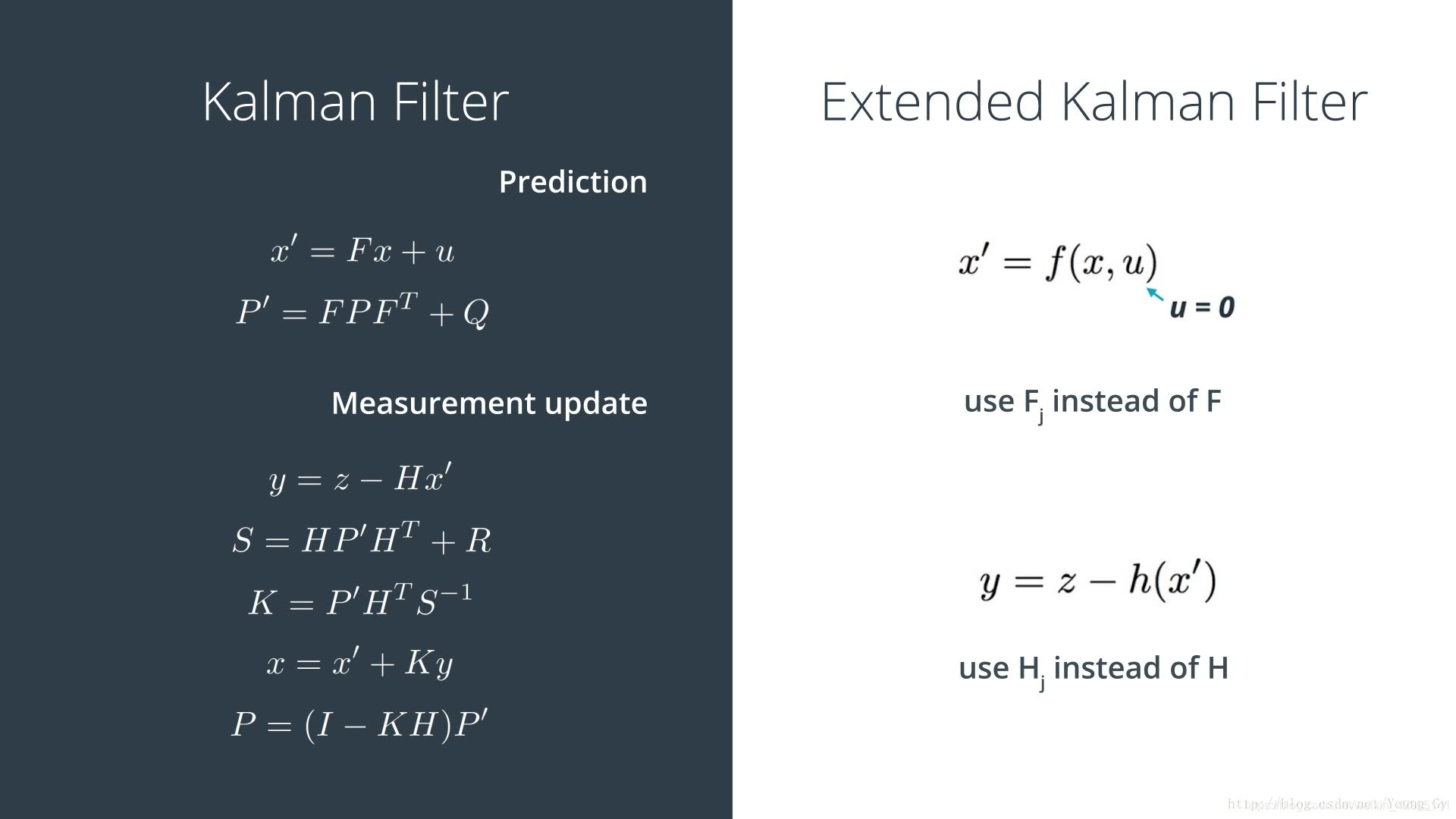
主要区别是:
- 在计算P ’ 时,F矩阵将被Fj代替。
- 当计算S,K和P时,卡尔曼滤波器中的H矩阵将被雅可比矩阵Hj代替。
- 为了计算x ',使用预测更新函数f代替F矩阵。
- 为了计算y,使用h函数代替H矩阵。
其中,非线性函数f(x,u),h(x′)f(x,u),h(x^′)f(x,u),h(x′)用非线性得到了更精准的状态预测值、映射后的测量值;线性变换Fj,Hj通过线性变换使得变换后的x,z仍满足高斯分布的假设。
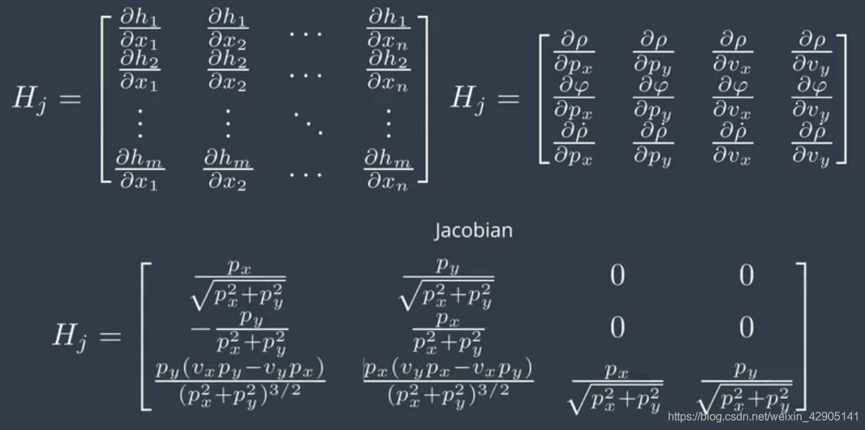
Fj,HjF_j,H_jFj,Hj计算方式如下:
Fj=∂f(x,u)x F_{j}=\frac{\partial f(x,u)}{x}Fj=x∂f(x,u)
Hj=∂h(x′)x H_{j}=\frac{\partial h(x^{'})}{x}Hj=x∂h(x′)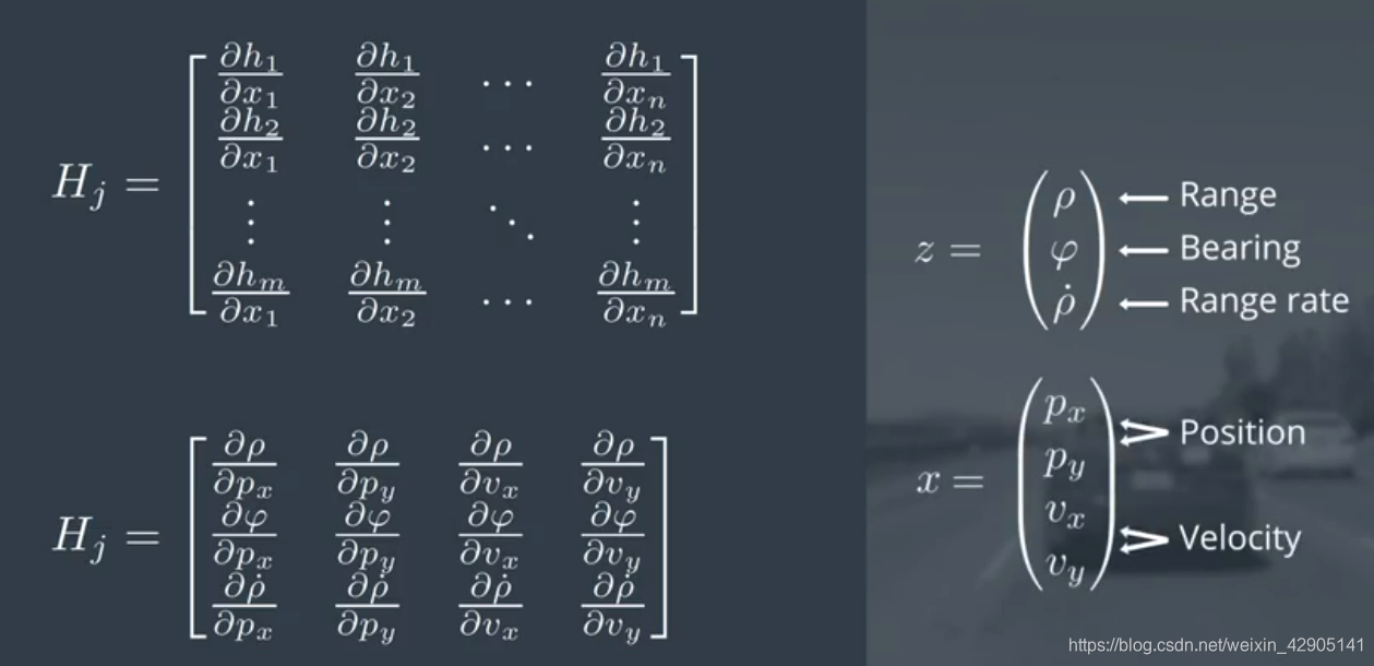
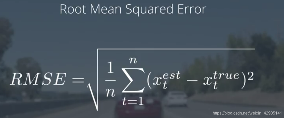
均方根值误差
kalman_filter.h
#ifndef KALMAN_FILTER_H_
#define KALMAN_FILTER_H_
#include "Eigen/Dense"

class KalmanFilter {
public:

  // state vector
  Eigen::VectorXd x_;

  // state covariance matrix
  Eigen::MatrixXd P_;

  // state transition matrix
  Eigen::MatrixXd F_;

  // process covariance matrix
  Eigen::MatrixXd Q_;

  // measurement matrix
  Eigen::MatrixXd H_;

  // measurement covariance matrix
  Eigen::MatrixXd R_;

  /**
   * Constructor
   */
  KalmanFilter();

  /**
   * Destructor
   */
  virtual ~KalmanFilter();

  /**
   * Init Initializes Kalman filter
   * @param x_in Initial state
   * @param P_in Initial state covariance
   * @param F_in Transition matrix
   * @param H_in Measurement matrix
   * @param R_in Measurement covariance matrix
   * @param Q_in Process covariance matrix
   */
  void Init(Eigen::VectorXd &x_in, Eigen::MatrixXd &P_in, Eigen::MatrixXd &F_in,
      Eigen::MatrixXd &H_in, Eigen::MatrixXd &R_in, Eigen::MatrixXd &Q_in);

  /**
   * Prediction Predicts the state and the state covariance
   * using the process model
   * @param delta_T Time between k and k+1 in s
   */
  void Predict();

  /**
   * Updates the state by using standard Kalman Filter equations
   * @param z The measurement at k+1
   */
  void Update(const Eigen::VectorXd &z);

  /**
   * Updates the state by using Extended Kalman Filter equations
   * @param z The measurement at k+1
   */
  void UpdateEKF(const Eigen::VectorXd &z);

  /**
  * A helper method to normalize the difference angle.
  */
  void  NormalizeAngle(double& phi);


};

#endif /* KALMAN_FILTER_H_ */
FusionEKF.h
#include "kalman_filter.h"
#include "tools.h"

using Eigen::MatrixXd;
using Eigen::VectorXd;

KalmanFilter::KalmanFilter() {}

KalmanFilter::~KalmanFilter() {}

void KalmanFilter::Init(VectorXd &x_in, MatrixXd &P_in, MatrixXd &F_in,
                        MatrixXd &H_in, MatrixXd &R_in, MatrixXd &Q_in) {
  x_ = x_in;
  P_ = P_in;
  F_ = F_in;
  H_ = H_in;
  R_ = R_in;
  Q_ = Q_in;
}

void KalmanFilter::Predict() {
  /**
  TODO:
    * predict the state
  */
	x_ = F_ * x_;
	MatrixXd Ft = F_.transpose();
	P_ = F_ * P_ * Ft + Q_;
}

void KalmanFilter::Update(const VectorXd &z) {
  /**
  TODO:
    * update the state by using Kalman Filter equations
  */
	VectorXd z_pred = H_ * x_;
	VectorXd y = z - z_pred;
	MatrixXd Ht = H_.transpose();
	MatrixXd S = H_ * P_ * Ht + R_;
	MatrixXd Si = S.inverse();
	MatrixXd PHt = P_ * Ht;
	MatrixXd K = PHt * Si;

	//new estimate
	x_ = x_ + (K * y);
	long x_size = x_.size();
	MatrixXd I = MatrixXd::Identity(x_size, x_size);
	P_ = (I - K * H_) * P_;
}

void KalmanFilter::UpdateEKF(const VectorXd &z) {
  /**
  TODO:
    * update the state by using Extended Kalman Filter equations
  */
	float px = x_(0);
	float py = x_(1);
	float vx = x_(2);
	float vy = x_(3);

	float rho = sqrt(px*px + py*py);
	float theta = atan2(py, px);
	float rho_dot = (px*vx + py*vy) / rho;
	VectorXd z_pred = VectorXd(3);
	z_pred << rho, theta, rho_dot;

	VectorXd y = z - z_pred;

	NormalizeAngle(y(1));

	MatrixXd Ht = H_.transpose();
	MatrixXd S = H_ * P_ * Ht + R_;
	MatrixXd Si = S.inverse();
	MatrixXd PHt = P_ * Ht;
	MatrixXd K = PHt * Si;

	//new estimate
	x_ = x_ + (K * y);
	long x_size = x_.size();
	MatrixXd I = MatrixXd::Identity(x_size, x_size);
	P_ = (I - K * H_) * P_;

}

void KalmanFilter::NormalizeAngle(double& phi) {
	/**
	TODO:
	* Normalize the difference angle between -pi to pi.
	*/
	phi = atan2(sin(phi), cos(phi));
}
FusionEKF.cpp
#ifndef FusionEKF_H_
#define FusionEKF_H_

#include "measurement_package.h"
#include "Eigen/Dense"
#include <vector>
#include <string>
#include <fstream>
#include "kalman_filter.h"
#include "tools.h"

class FusionEKF {
public:
  /**
  * Constructor.
  */
  FusionEKF();

  /**
  * Destructor.
  */
  virtual ~FusionEKF();

  /**
  * Run the whole flow of the Kalman Filter from here.
  */
  void ProcessMeasurement(const MeasurementPackage &measurement_pack);

  /**
  * Kalman Filter update and prediction math lives in here.
  */
  KalmanFilter ekf_;

private:
  // check whether the tracking toolbox was initialized or not (first measurement)
  bool is_initialized_;

  // previous timestamp
  long long previous_timestamp_;

  // tool object used to compute Jacobian and RMSE
  Tools tools;
  Eigen::MatrixXd R_laser_;
  Eigen::MatrixXd R_radar_;
  Eigen::MatrixXd H_laser_;
  Eigen::MatrixXd Hj_;
  Eigen::MatrixXd Pfusion_;
  Eigen::MatrixXd Ffusion_;
  Eigen::MatrixXd Qfusion_;
  Eigen::VectorXd xfusion_;

  float noise_ax = 0.0;
  float noise_ay = 0.0;


};

#endif /* FusionEKF_H_ */
#include "FusionEKF.h"
#include "tools.h"
#include "Eigen/Dense"
#include <iostream>

using namespace std;
using Eigen::MatrixXd;
using Eigen::VectorXd;
using std::vector;

/*
 * Constructor.
 */
FusionEKF::FusionEKF() {
  is_initialized_ = false;

  previous_timestamp_ = 0;

  // initializing matrices
  R_laser_ = MatrixXd(2, 2);
  R_radar_ = MatrixXd(3, 3);
  H_laser_ = MatrixXd(2, 4);
  Hj_ = MatrixXd(3, 4);
  Pfusion_ = MatrixXd(4, 4);
  Ffusion_ = MatrixXd(4, 4);
  Qfusion_ = MatrixXd(4, 4);
  xfusion_ = VectorXd(4);


  //measurement covariance matrix - laser
  R_laser_ << 0.0225, 0,
        0, 0.0225;

  //measurement covariance matrix - radar
  R_radar_ << 0.09, 0, 0,
        0, 0.0009, 0,
        0, 0, 0.09;

  /**
  TODO:
    * Finish initializing the FusionEKF.
    * Set the process and measurement noises
  */
  H_laser_ << 1, 0, 0, 0,
	  0, 1, 0, 0;

  xfusion_ << 1, 1, 1, 1;
  Pfusion_<< 1, 0, 0, 0,
	  0, 1, 0, 0,
	  0, 0, 100, 0,
	  0, 0, 0, 50;

  Ffusion_ << 1, 0, 0, 0,
	  0, 1, 0, 0,
	  0, 0, 1, 0,
	  0, 0, 0, 1;

  Qfusion_ << 0, 0, 0, 0,
	  0, 0, 0, 0,
	  0, 0, 0, 0,
	  0, 0, 0, 0;

  noise_ax = 9.0;
  noise_ay = 9.0;
}

/**
* Destructor.
*/
FusionEKF::~FusionEKF() {}

void FusionEKF::ProcessMeasurement(const MeasurementPackage &measurement_pack) {


  /*****************************************************************************
   *  Initialization
   ****************************************************************************/
  if (!is_initialized_) {
    /**
    TODO:
      * Initialize the state ekf_.x_ with the first measurement.
      * Create the covariance matrix.
      * Remember: you'll need to convert radar from polar to cartesian coordinates.
    */
    // first measurement
    cout << "EKF: " << endl;
	//kf_.x_ = VectorXd(4);
	//ekf_.x_ << 1, 1, 1, 1;

    if (measurement_pack.sensor_type_ == MeasurementPackage::RADAR) {
      /**
      Convert radar from polar to cartesian coordinates and initialize state.
      */
		const float m1 = measurement_pack.raw_measurements_[0] * cos(measurement_pack.raw_measurements_[1]);
		const float m2 = measurement_pack.raw_measurements_[0] * sin(measurement_pack.raw_measurements_[1]);
		const double vx = measurement_pack.raw_measurements_[2] * cos(measurement_pack.raw_measurements_[1]);
		const double vy = measurement_pack.raw_measurements_[2] * sin(measurement_pack.raw_measurements_[1]);
		xfusion_ << m1, m2, vx, vy;
		ekf_.Init(xfusion_, Pfusion_, Ffusion_, Hj_, R_radar_, Qfusion_);
    }
    else if (measurement_pack.sensor_type_ == MeasurementPackage::LASER) {
      /**
      Initialize state.
      */
		xfusion_ << measurement_pack.raw_measurements_[0], measurement_pack.raw_measurements_[1], 0, 0;
		ekf_.Init(xfusion_, Pfusion_, Ffusion_, H_laser_, R_laser_, Qfusion_);
    }


	previous_timestamp_ = measurement_pack.timestamp_;
    // done initializing, no need to predict or update
    is_initialized_ = true;
    return;
  }

  /*****************************************************************************
   *  Prediction
   ****************************************************************************/

  /**
   TODO:
     * Update the state transition matrix F according to the new elapsed time.
      - Time is measured in seconds.
     * Update the process noise covariance matrix.
     * Use noise_ax = 9 and noise_ay = 9 for your Q matrix.
   */

  float dt = (measurement_pack.timestamp_ - previous_timestamp_) / 1000000.0; //dt - expressed in seconds
  if (dt == 0) {
	  return;
  }
  previous_timestamp_ = measurement_pack.timestamp_;

  ekf_.F_ << 1, 0, dt, 0,
	  0, 1, 0, dt,
	  0, 0, 1, 0,
	  0, 0, 0, 1;

  //2. Set the process covariance matrix Q
  ekf_.Q_ << (pow(dt, 4) / 4)* noise_ax, 0, (pow(dt, 3) / 2)* noise_ax, 0,
	  0, (pow(dt, 4) / 4)* noise_ay, 0, (pow(dt, 3) / 2)* noise_ay,
	  (pow(dt, 3) / 2)* noise_ax, 0, pow(dt, 2)* noise_ax, 0,
	  0, (pow(dt, 3) / 2)* noise_ay, 0, pow(dt, 2)* noise_ay;

  ekf_.Predict();

  /*****************************************************************************
   *  Update
   ****************************************************************************/

  /**
   TODO:
     * Use the sensor type to perform the update step.
     * Update the state and covariance matrices.
   */

  if (measurement_pack.sensor_type_ == MeasurementPackage::RADAR) {
    // Radar updates
	ekf_.R_ = R_radar_;
	ekf_.H_ = tools.CalculateJacobian(ekf_.x_);
	ekf_.UpdateEKF(measurement_pack.raw_measurements_);

  } else {
    // Laser updates
    ekf_.H_ = H_laser_;
	ekf_.R_ = R_laser_;

	ekf_.Update(measurement_pack.raw_measurements_);

  }

  // print the output
  cout << "x_ = " << ekf_.x_ << endl;
  cout << "P_ = " << ekf_.P_ << endl;
}

更多推荐


 7
7 0
0- 0


 已为社区贡献1条内容

所有评论(0)